Ncdf
Different Ways To Evaluate N(x) in Mathematica


Notes on Error & Efficiency
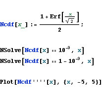
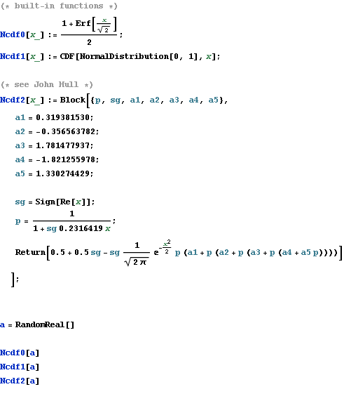
Using built-in function, one can obtain almost exact values.
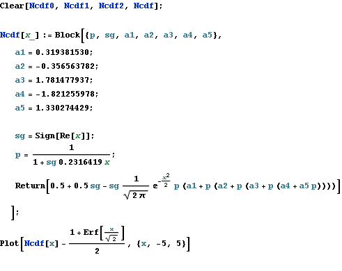
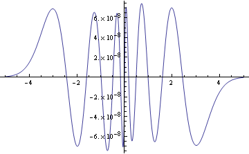
In constrast, the widely used approximation could introduce an errof of  , as shown in the figure.
But, as experiments show us, using built-in functions to evaluate N(x) is very inefficient.
If an algorithm involves N(x) frequently, and if one can withstand an error of  , the widely used approximation is a better choice.
More Efficiently
Recently I designed an algorithm that evaluates N(x) really frequently.
In this case, both of the above are not the best choice.
If one can withstand an error of  , keeping 1201 exact values of N(x) between [-6, 6] and using qudratic interpolation will work more efficiently.
When x is out of the interval [-6, 6], we set N(x) to 0 or 1.
The error caused in this part this is, as shown in the following computations, always less than  .
.
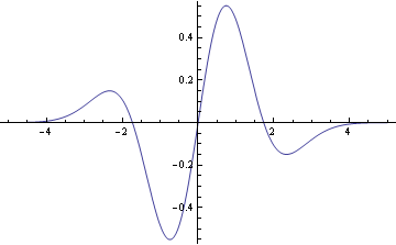
Besides, althought the error due to qudratic interpolations depends on the derivative of N(x), as shown in the figure, its absolute value is quite small.